example
The following example takes you step by step through an analysis using PERFORM. The following sections are found here.
A. Background
Aluminum lids are produced on a press which has 22 stations. Each day, lids from each station are sampled and the lid height is measured. Each sample contains a single lid from each station. Data are collected over a three-month period. The specifications for this characteristic are 98 ± 5.
B. Loading the Data
The Data have been loaded into a file called example.mvp. This file contains three columns of data. The first column contains the Sample numbers (1-134). The second column contains the Station numbers (1-22). The third column contains the Height measurements. (See Data File Layout.)
From the Main Form menu, select File|Open and load the file example.mvp. The Data Editor will appear as follows. (See Data Editor Overview.)
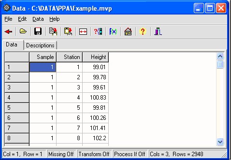
The variable names are seen at the top of the columns of the Data Grid. From this bottom of this form, it can be seen that there three columns and 2948 rows.
Click the ![]() speed button to return to the Main Form.
speed button to return to the Main Form.
C. Setting-up the Main Form
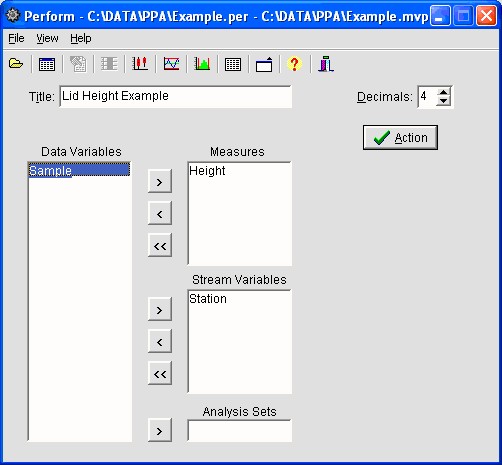
- Enter a tile into the Title Box as "Lid Height example". (See Main Form.)
- Enter the specifications into the Specification Edit Boxes (98 ± 5 which equates to a USL of 103, a target of 98, and a LSL of 93).
- Select the variable Height, and move it into the Measures box.
- Select the variable Station, and move it into the Grouping Variables box.
The Main Form should appear as follows.
D. Histogram
To view a Histogram of the combined data, click the ![]() speed button on the Main Form. The following Histogram will be displayed. (See histograms Form.)
speed button on the Main Form. The following Histogram will be displayed. (See histograms Form.)
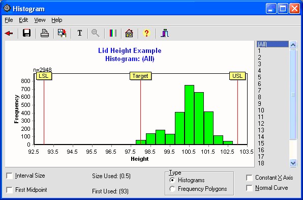
Note the appearance of the Histogram. (See What is a Histogram?)
Click the ![]() speed button to hide the Histogram and return to the Main Form.
speed button to hide the Histogram and return to the Main Form.
E. Box & Whisker Plots
To view Box & Whisker Plots by Station, Click the ![]() speed button on the Main Form. The following Box & Whisker Plot will be displayed. (See Box & Whisker Plots Form.)
speed button on the Main Form. The following Box & Whisker Plot will be displayed. (See Box & Whisker Plots Form.)
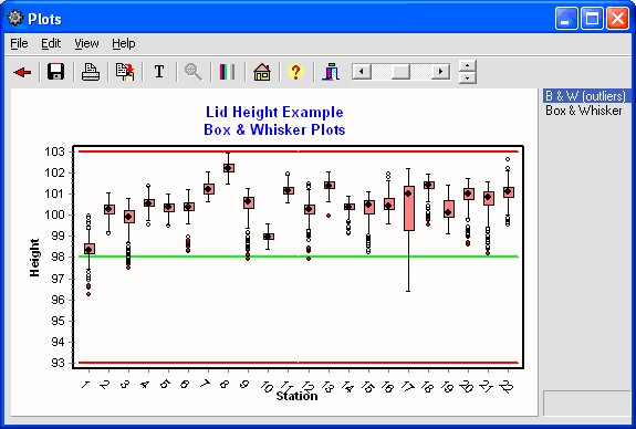
Click on the B&W(Outliers) to see the Box & Whisker Plots with outliers. (See What are Box & Whisker Plots?)
Click the ![]() speed button hide the Box & Whisker Plots and return to the Main Form.
speed button hide the Box & Whisker Plots and return to the Main Form.
F. Control-Charts
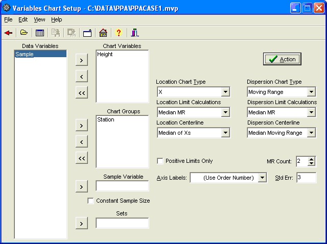
For individual observations per process stream, as in this case, you will want to display the charts using X-Charts by Station. Click the ![]() speed button on the Main Form. In the Variables Control Chart Setup Form, use the following setup. (See What are Control Charts?)
speed button on the Main Form. In the Variables Control Chart Setup Form, use the following setup. (See What are Control Charts?)
The following X and Moving Range Chart form will be displayed. (See Variables Control Chart Form.)
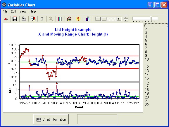
Select the numbers on the right side of the Chart to see X-Charts for each Station.
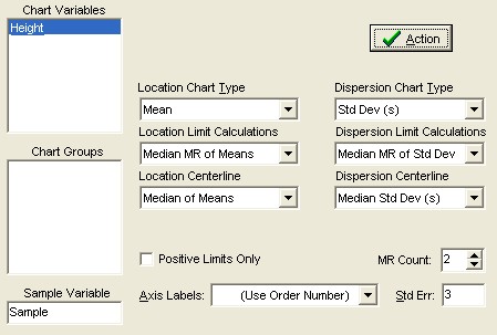
You may also wish to see the stations combined together. This can be done using a Mean and Standard Deviations Chart (X-bar and s chart). We will do this by selecting "sample" as the sample variable. Within each sample are multiple stations, so we cannot use typical control limits calculations. We will create limits using the Moving Range of the means and standard deviations. Set this up as follows.
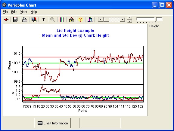
You will then see the following chart displayed.
G. Run-Charts
Run charts are simply through-time plots of data without control limits. In this example, we will want to see the Run chart with the specifications.
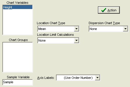
First set up the chart using the folowing on the Variables Control Chart Setup Form.
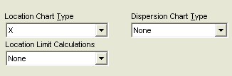
Next, select "Show Specifications" from the View Menu on the Variables Chart Form.
The Control Chart form will now display Run charts using the Specification limits.
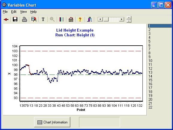
Select the numbers on the right side of the Chart to see Run Charts for each Station compared against the specifications and target.
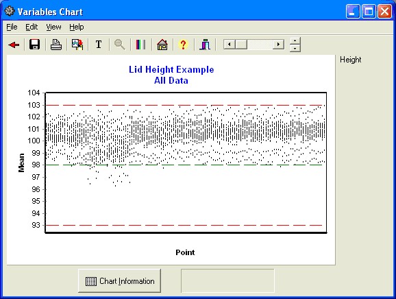
H. All Data Points Chart
In this output, we want to see all data points from the 22 stations on one chart. Set up the Control chart in the following manner.
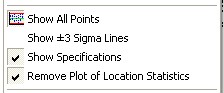
Next from the View Menu select the following Options. (Show All Points, Show Specifications, and Remove Plot of Location Statistics.)
Your chart will now appear as follows. This chart is useful to see the distribution moving through time.
I. Graphics Discussion
The graphical analysis suggests an off-target condition is clearly present as seen in the histogram. The box plots also show significant differences between stations.
The combined data run chart gives a sense of the data through time. A slight change occurred one-fourth of the way through the period, but then stabilized into a consistent pattern.
The X-Charts suggest that the individual stations are not stable through time. When compared against the specification ranges, though, the through-time variation observed appears to be minimal.
J. Performance Analysis
Click the ![]() button on the Main Form. This will process the data and generate the Process Performance Analysis.
button on the Main Form. This will process the data and generate the Process Performance Analysis.
The Text Output Form will be displayed as follows. (See Text Output Form.)
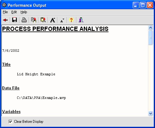
Here is the text output.
PROCESS PERFORMANCE ANALYSIS
1/20/2007
Title
Lid Height example
Data File
C:\Program Files\MVP Programs\Perform\example.mvp
Variables
	Measures:
		Height

	  Groups:
		Station  1 to 22
Specifications
	   USL = 103.0000
	Target = 98.0000
	   LSL = 93.0000
Process Stream Analysis
Group    n      Mean       Low      High   Range     Std  Std(MMR)
    1  134   98.3680   96.2600   99.9800  3.7200  0.6277   0.2621
    2  134  100.2191   99.1500  101.0800  1.9300  0.4049   0.2411
    3  134   99.7260   97.4800  100.7900  3.3100  0.7662   0.2621
    4  134  100.5613   99.5500  101.3900  1.8400  0.2877   0.2201
    5  134  100.3560   99.5000  100.9900  1.4900  0.2942   0.2306
    6  134  100.2869   98.2900  101.2100  2.9200  0.5854   0.2411
    7  134  101.2243  100.6300  102.0600  1.4300  0.3257   0.2411
    8  134  102.2103  101.5000  102.9400  1.4400  0.3178   0.2621
    9  134  100.3425   97.9300  101.2600  3.3300  0.7890   0.1782
   10  134   98.9664   98.3800   99.5800  1.2000  0.2402   0.1468
   11  134  101.1778  100.6100  101.9400  1.3300  0.2578   0.2096
   12  134  100.1609   97.9300  101.4800  3.5500  0.6743   0.2516
   13  134  101.3817   99.9400  102.0600  2.1200  0.2798   0.2411
   14  134  100.3308   99.1500  100.9300  1.7800  0.3427   0.2306
   15  134  100.2666   98.2600  101.1400  2.8800  0.6785   0.2306
   16  134  100.5613   99.5900  101.9400  2.3500  0.4530   0.1887
   17  134  100.4739   96.4100  102.2000  5.7900  1.2723   0.2306
   18  134  101.3035   99.5500  101.9600  2.4100  0.4947   0.2201
   19  134  100.2491   99.1500  101.4300  2.2800  0.5375   0.2096
   20  134  100.7978   98.6100  101.7600  3.1500  0.7122   0.2411
   21  134  100.5726   98.1900  101.6100  3.4200  0.7952   0.2725
   22  134  101.0587   99.5300  102.6300  3.1000  0.4902   0.2725

	SQRT(MSW) = Avg Std Dev within = 0.5823
	AVG Std(MMR) = Avg Std Dev from Median Moving Range = 0.2311
Descriptives
	       n = 2948
	    Mean = 100.4816
	Std. Dev = 0.9788
	     Low = 96.2600
	      Q1 = 100.0625
	  Median = 100.5900
	      Q3 = 101.1400
	    High = 102.9400
	Skewness = -0.732
	Kurtosis = 0.759
Variance Components
	Total Variance About Target = 7.1165  100.00%
	        Off-target Variance = 6.1584   86.54%
	         Potential Variance = 0.0534    0.75%
	    Process Stream Variance = 0.6190    8.70%
	     Time(Control) Variance = 0.2856    4.01%
Performance
	%Off-Target = 24.82%
	Max Stream Mean = 102.2103
	Min Stream Mean = 98.3680
	%Process Stream Difference = 38.42%

	ppk       = 0.858
	ppm       = 0.625
	pp        = 1.703
	pp(Stream)= 2.862
	Cp(pot)   = 7.212

	n = 2948
	Above USL = 0
	Below LSL = 0
	Total Out = 0
	(0 ppm)
Click the ![]() speed button return to the Main Form.
speed button return to the Main Form.
K. Performance Text Output Discussion
For each of the 22 stations, descriptive statistics are generated including the mean, standard deviation, low, high, and range. In addition, since individual readings are taken in time order, a standard deviation is generated using the median moving range for each station.
The performance measure, ppm was 0.625. pp was 1.703. This suggests a large loss in performance because of lack of targeting. In addition, 38.42% of the specification range is taken up by station to station differences. This could also be thought of as a station targeting issue. This can be seen graphically in the histogram and the box plots.
L. Performance Analysis Charts
To view the Performance Analysis Charts, click the ![]() speed button on the Main Form. The following Performance Analysis Chart Form will be displayed. (See Performance Charts Form.)
speed button on the Main Form. The following Performance Analysis Chart Form will be displayed. (See Performance Charts Form.)
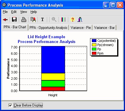
Click the Tabs on the Top of this form to view each of the Performance Analysis Charts.
M. Conclusions
From this analysis, it can be seen that the biggest opportunity comes from getting the individual stations on target. While improvement in control will minimize variation, the through-time sources of variability do not represent the largest opportunity. Measurement error analysis is not shown, but from the process potential assessment, measurement error may be considered negligible.
These results are typical of many observed processes. Improvements in targeting and reduction of tool-to-tool or station-to-station differences often represent an important opportunity. While improvement in through-time stability or control does not represent a large improvement opportunity in this case, it may be critical in others.
