Normality Testing Guidelines
The Normal, Gaussian, or sometimes called bell-shaped distribution, is one of the most important distributions because of its wide range of practical applications. Because normality is a critical assumption which underlies the use of many statistical tests and inferences, it is an assumption which must be checked.
MVPstats provides four different procedures for testing the assumption of normality. Included are the Anderson-Darling test statistic, the Shapiro-Wilk test statistic, the Lin-Mudholkar test statistic, and Skewness and Kurtosis indices.
There is probably no distribution which can be said to be perfectly normal. The question one usually asks, however, is whether or not the population from which a data set has been drawn can be adequately modeled with the normal distribution for the intended purpose. The appropriateness of the model is critical in process capability analysis and also many statistical tests.
The assumption of normality must be tested objectively. Looking at a histogram and making the statement, ''It looks normal to me,'' does not provide conclusive evidence that the normal assumption holds. A leptokurtic distribution looks symmetric and bell-shaped, but it is not normal.
Many industrial applications have underlying process distributions that are not normally distributed. The process may be better modeled with an exponential, Weibull, Johnson, or some other distribution. The data may come from a process which is not in state of statistical control, yielding no valid underlying distribution (in which case underlying distributional analysis would be completely inappropriate).
Power in a test for normality is the ability of the test to detect the presence of a non-normal distribution. The power to detect non-normal distributions varies with the test that is used. Each of the tests for normality also vary in their ability to detect different types of departures from normality.
Powerful tests with very large sample sizes will reject the normality assumption with only slight deviations from normality. This rejection may or may not answer the question of whether or not the normal approximation is adequate. Judgement is required.
Anderson-Darling is one of the most powerful statistics for detecting most departures from normality. It may be used with small sample sizes (n=7). Very large sample sizes may reject the assumption of normality with only slight imperfections. But, industrial data with sample sizes of 200 and more, have easily passed the Anderson-Darling test.
Shapiro-Wilk is similar in power to Anderson-Darling, with Shapiro-Wilk having a slight edge in many situations. You will find very similar results between these two tests.
Lin-Mudholkar, generally is the next most powerful test after Anderson-Darling and Shapiro-Wilk, depending on the type of departure from normality. It is only sensitive in detecting non-symmetrical departures from normality. In fact, for departures of normality due to skewness, the Lin-Mudholkar test is more powerful than Anderson-Darling or Shapiro-Wilk. Lin-Mudholkar can be used with a sample of size as low as ten.
Skewness and Kurtosis should generally be used with larger sample sizes. They are generally lower in power than the other tests. They can be used with smaller sample sizes, but have little power, so only rejection would have meaning. Since they have little power, if you accept the assumption of normality with a small sample size, the evidence for normality is still inconclusive.
Skewness and Kurtosis are powerful in their ability to detect outliers. Skewness and Kurtosis, in cases where the data set contains extreme values, may reject normality even before Anderson-Darling. A data set was collected from a normal distribution, with a sample of size 50. All test statistics from the data set showed the distribution to be normal. A single point was then added to the data set four to five standard deviations away from the mean. Skewness and Kurtosis rejected the assumption of normality while Anderson-Darling passed it!
Skewness and Kurtosis indices can also provide some clues as to why other procedures rejected the assumption of normality. histograms and Box and Whisker plots also give some insight into data, as well as visual comparison between data sets.
Some statisticians recommend using different tests for different ranges of sample sizes. The idea is to use tests with more power for smaller sample sizes. This would avoid using powerful tests for large sample sizes which reject the assumption of normality due to unimportant discrepancies. One must be cautioned in this approach because there is no one test which is most powerful in all cases. As the type of departure changes so do the powers of each of the normality test statistics. It is recommended, when using MVPstats, to simply run all tests and examine the results and make comparisons.
Anderson-Darling and Shapiro-Wilk can be examined first, even with larger sample sizes, and if it passes with large sample sizes, the population from which the data set was drawn is probably very close to normal.
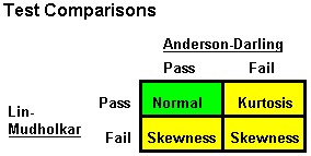
Lin-Mudholkar can be examined next and comparisons can be made with Anderson-Darling. Rejection by Lin-Mudholkar and not by Anderson-Darling may mean your distribution is skewed. On the other hand, Lin-Mudholkar is not sensitive to non-normal symmetrical distributions, so comparison is needed with Anderson-Darling.
Anderson-Darling and the Lin-Mudholkar tests when used together may provide some clues for the type of departure from normality as follows:
The Skewness and Kurtosis indices can then be examined. As mentioned previously, these statistics can provide clues as to why other procedures rejected the assumption of normality, but are generally weak for small sample sizes.
Sometimes, histograms will visually portray why the assumption of normality was rejected or the reasonableness of the normality assumption.
Many of the tests for normality will fail when you have inadequate measurement resolution. If your histogram displays only two intervals for your sample, you will not pass the tests found in MVPstats. This DOES NOT mean that you do not have an underlying normal distribution, it means you do not have any ability to judge what kind of distribution you have. You will get into trouble when you drop down to only two or three intervals in attempting to determine what type of underlying distribution you have.
If the data are time ordered, a run chart or X-chart should also be examined to check for lack of stability. This should be done before any distributional test is conducted.
A final caution, the reasonableness of the assumption of normality should be checked. A data set with a sample of size 40, easily passed Anderson-Darling, Lin-Mudholkar, and the Skewness and Kurtosis tests. It had a mean of 5150 and a standard deviation of 2054. But notice that three standard deviations below the mean is equal to -1012. Since these values come from a process that is impossible to fall below zero, the assumption of normality is not reasonable.
